Earthquake Damage Prediction with Machine Learning — Part 3
By — Jen Neng Ng

This story is continue from a Series of :
Part 4: Implementation (Continue)
Part 3: Implementation
Data Splitting

The data split created 146590 rows train dataset and 36506 rows test dataset.
Data Cleaning
Use the boxplot to trim the outlier:

Data Sampling
We can check the ratio of each class in damage_grade:

Let’s use the SmoteClass library to perform upsampling for imbalance class:
After perform upsampling, each class should be balanced:

Data Transformation & Scaling
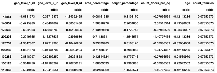
We can use one-hot encoding to encode category data and scaling for numeric rescale

Experiment Plan
Based on the previous related work analysis (Part 1), we can choose a minimum of three machine learning models for the experiment. The best to compare is XGBoost, Random Forest, and Decision Tree for learning purposes. By comparing these three “tree” model, it provides a basic understanding of bagging and boosting from one use case.
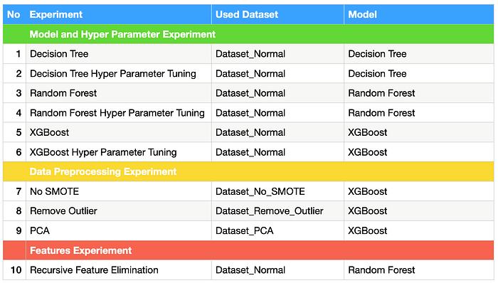
In this experiment plan, we will try to find out whether upsampling imbalance class, remove outlier, and PCA transformation will help to increase the dataset prediction accuracy or not. Bear in mind that, every dataset (training/validation/test) has its own data distribution, not every model must apply a particular process or procedure.
The experiment plan can be conducted as:

Decision Tree
The implementation of the decision tree method will be using rpart package, it is a widely used package for Classification & Regression Tree (CART) modeling.
Experiment 1
The dependent variables have assigned as a factor for classification. The min split here refers to the minimum observations count exists in a node required when splitting. min bucket means the minimum observations count require in any terminal node. The minbucket=10 provided in the model is to avoid overfitting happen where it could prevent a few of the observations from trying to create a new tree along the way. The cp value here refers to the complexity parameter, it controls the overall decision tree size. By assigned it to a negative amount, it will generally let the tree be fully grown.

The result has surprised us, by just using 197 seconds training time, it has 0.749 accuracy outcome. The output also measure that class 2 have the highest accuracy rate
The plot above indicate 2000 tree is enough for the model.

The top important variable ranking plot has measured that most of the numeric continuous variables are important.
Experiment 2 (Tuning)
Now, we will use parameter searching from caret train function to find the optimal parameter. Take a close look in caret package tuning document, the rpart package only supports cp (Complexity Parameter) as the tuning target.


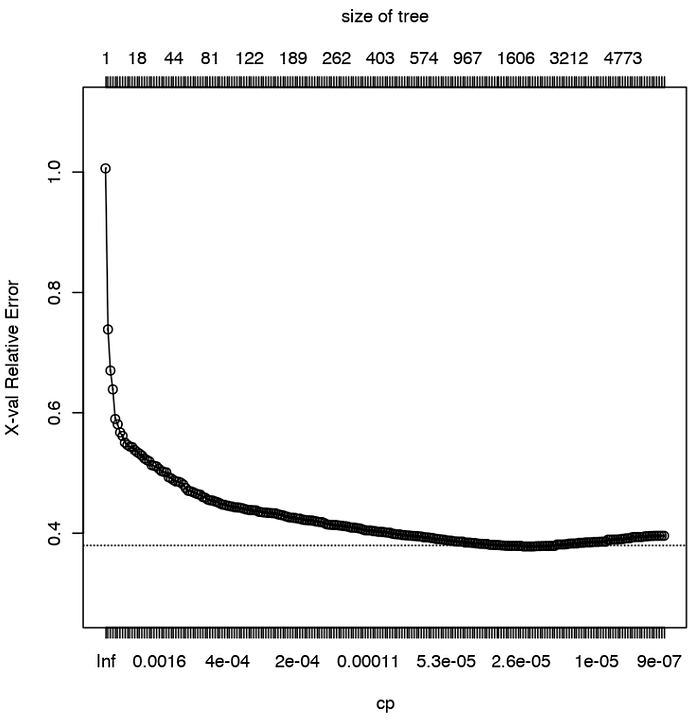
The plot above is the outcome of caret train model, it measures the best accuracy that can be obtained when cp value is closed to zero.
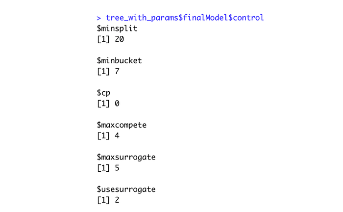
We can peak on the other parameter values from the tuned model
Lets put in the parameter result to a new model:


The result shows that the accuracy is lower (-0.12) than previously. It may be the cp value is not suitable for this dataset. In the previous complexity parameter plot, it measures that the accuracy can reach 0.66 above by using cross-validation on the training dataset. By comparing to the test dataset accuracy, the accuracy is slightly lower (0.62). In general, increasing the cp will provide more generalisation for the test dataset. Mean the model can be more generalisation and obtain similar accuracy for different data.
In this case, the test dataset maybe is more similar to a training dataset where increase cp to increase generalisation does not provide a better outcome.
Adjusting back the cp value to -1 may have different finding:

The F1 score is similar to Experiment 1 model (0.749). Even though the parameter min split and min bucket have changed to 20 and 7.
Random Forest
Random Forest is an ensemble bagging model. It generally builds a lot of decision tree parallelly with random sub-samples, then the model prediction will calculate the most frequent class as the answer. In that way, random forest will get lower variance compared to decision tree because decision tree is more sensitive to specific data and only one single decision tree is built. Moreover, random forest will get less overfit issues even though the number of trees is increased. For the implementation part, there are two popular packages in R can be used for random forest model which is cForest and randomForest package. In these experiments, randomForest will be used, because it is performing faster compare to cForest.
Experiment 3
In randomForest function, it allows setting the number of trees, sample size, and the number of variables at each splitting tree node (mtry) for the model parameter. As randomForest model require a long time to train, the experiment will use a low number of tree and sample size.


The accuracy is 0.624, which is quite low compare to decision tree kernel especially the Class 1 prediction. Also, it consumes a lot of processing time when training the kernel.

The model plot also shows the error doesn’t increase even though the number of trees is increasing.
Experiment 4 (Tuning)
According to the document at caret documentation, the caret train function support mtry parameter for parameter tuning only. For this experiment, it will only look for the best mtry number in parameter tuning.
the implementation will randomly select 5000 samples and use the out-of-bag method to determine the error.
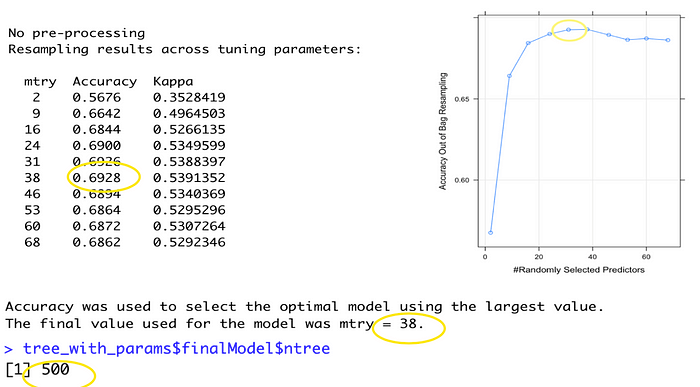
The plot above shows the accuracy could improve a lot if mtry is increasing. The best optimal value for mtry and ntree is 38 and 500.
Let’s fit the optimal parameter to a new model:

The micro F1 score has increased by 0.05 compared to Experiment 3 (0.624). The obtained testing score 0.677 is similar to the training validation score (0.6928), which means the dataset difference doesn’t affect the model performance. On the other hand, the processing time also increased from 98 seconds to 2000 seconds as the numbers of trees and mtry increase. It is quite high compare to the decision tree model.
XGBoost
Extreme Gradient Boosting (XGB) is a popular boosting model. It is an ensemble gradient boosting model that combines the bagging and gradient boosting techniques. It generally boosting the weak learners by trying to reduce the training error. In R, it has an XGBoost package that supports the model implementation.
Experiment 5

There are several model parameters for XGBoost such as eta (learning rate), max_depth, nround, subsample, colsample_bytree, and gamma (min_split_loss). It also indicates that the train-merror has further reduced the error after every single round.
The micro F1 score is 0.7494, which is slightly higher than the decision tree and random forest by just using 147 seconds of training time. Also, the class 1 prediction model accuracy and Specificity is getting the highest score (0.676) compare to others model. As the dependent variable class 1 is having lesser observations compare to the other two classes, it is noticeable that the XGBoost has improved the accuracy of the weak learner class.
Experiment 6 (Tuning)
In this experiment, there will be different group values for these five parameters. As the processing time took too long, the observation count has reduced to 1000.

The max_depth from the grid search result is very low(max_depth=2). According to the nround and accuracy record in the yellow circuit, it can be assumed that increasing the nrounds will improve the accuracy.
Let’s fit the optimal parameter found to a new model:


It shows that the accuracy has dropped compared to Experiment 5 (0.7497), it could be due to the eta (learning rate) are setting higher and max_depth are setting lower compare to previous.
Thus, let’s adjust back the eta and max_depth and observe the results:

After adjusting the eta and max_depth back to Experiment 5 model value, the micro F1 score has boosted to 0.8775, and it is close to the training score 0.943 (train- merror:0.0571). The document on XGBoost documentation also warns the user that increasing the max_depth value will make the model more complex and easy to overfit. But in this model, it does not seem to overfit too much. Nevertheless, The score for each class listed also indicate the accurate rate is well balanced in this model.
Conclusion & Summary (Experiment 1~6)
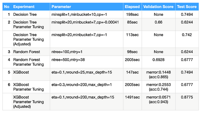
In conclusion, the decision tree and random forest from rpart didn’t provide too much parameter for tuning. The experiments also prove that the optimal value obtains from caret train function doesn’t make the model adopt the test dataset better. (test score is lowering) On the other hand, increasing depth and create more trees are benefiting both train and test dataset.
Experiment 3 and 4 also prove that random forest is the most stable kernel, the validation and test score is almost the same. However, random forest did consume too much training time. I have tried to run random forest in Python with the same dataset, it boosts the performance a bit compare to R. In most of the scenarios, Random forest can perform better than decision tree. Because I have limited the size of the sampling in this kernel, it has reduced both accuracy and time consumption.
As for XGBoost, it obtains the highest class 1 prediction score compare to the other two kernels. It is worth mentioning that it has improved weak learner prediction significantly.


